VLBI Reconstruction Dataset

EHT Imaging Challenge

Welcome to the Event Horizon Telescope Imaging Challenge Webpage! This challenge is meant to help us understand the performance of different imaging algorithms on future Event Horizon Telescope (EHT) data. We hope the results of the challenge will help us better understand the biases of each imaging algorithm, and aid in developing better methods.

Next Deadline: December 20, 2017

Testing Data and Submission Instructions

Data Parameters and Noise Properties

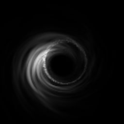
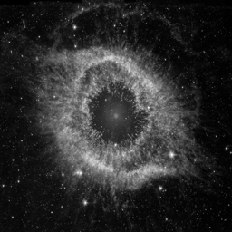
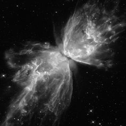
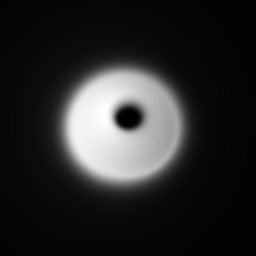
Sample Data With Ground Truth Images

Past Challenges

Data Formats and Conversion

Sample Imaging Script

Questions and Feedback

Testing Data and Submission Instructions

Download the test data from HERE.

Use your algorithm to generate an image for each of the data files. For each < filename >.txt file, submit a FITS image with the name < filename >.fits and the FOV specified in the README File. Further instructions can be found in the README file.

Submit your reconstructed images. Compress all of your reconstructed FITS images into a ZIP file. Submit this ZIP file with the required additional information.

Data Parameters and Noise Properties

Dataset Number	Source Location	Telescopes	Total Flux (Janskys)	Noise Property
1	Sgr A*	SMA, JCMT, SMT, LMT, ALMA, APEX, PV, SPT	2	Thermal & Atmospheric & Scattering
2	Sgr A*	SMA, JCMT, SMT, LMT, ALMA, APEX, PV, SPT	2	Thermal & Atmospheric & Scattering
3	Sgr A*	SMA, JCMT, SMT, LMT, ALMA, APEX, PV, SPT	2	Thermal & Atmospheric & Scattering

Thermal Noise

The standard deviation of thermal noise introduced in each measured visibility is fixed based on bandwidth ( $\nu$ ), integration time ( $\tau$ ), and each telescope’s System Equivalent Flux Density ( $\rho$ ). A factor of 1/0.88 is included due to the effect of 2-bit quantization.

$\sigma_{\mbox{\tiny{Thermal}}} = \frac{1}{0.88} \sqrt{ \frac{\rho_1 \rho_2}{ \Delta \nu \tau} }$ SEFDs for each site in the EHT are taken from here. The SEFDs used across different imaging challenges may change to reflect changes in the measured SEFDs.

Atmospheric Noise

Inhomogeneities in the atmosphere cause the light to travel at different velocities towards each telescope. The atmosphere affects an ideal visibility (spatial frequency measurement) by introducing an additional phase term:

$\Gamma_{k,j}^{\mbox{\tiny{measured}}} = e^{ i (\phi_k - \phi_j)} \Gamma_{k,j}^{\mbox{\tiny{ideal}}}$

where $\phi_k$ and $\phi_j$ are the phase delays introduced in the path to telescopes k and j respectively. A common technique to eliminate the effect of atmospheric errors is to use closure phases.

Systematic Noise

Systematic (site-based) gain errors are introduced as errors in the SEFD used for calibration. A common technique to eliminate the effect of gain errors is to use closure amplitudes.

For each site, the SEFD used for calibration is modeled as, constant SEFD adjusted for the observed (noisy) opacity provided in the data tables. For each scan, the true site SEFD (used to model the observed visibility signal-to-noise ratio) includes the following adjustments, all modeled as Gaussian random processes with 1-sigma values equal to:

10% constant SEFD variation for each site, plus 10% additional scan-by-scan variation
10% variation in the true opacity (relevant only to source attenuation, no specific modeling of sky temperature)

Time Varying

SgrA* is believed to change on the order of minutes. To simulate this effect observations taken over the course of the night are sampled from frames of a movie rather than a static image.

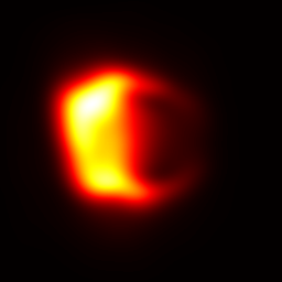
Sample Data With Ground Truth Images

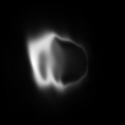
We provide a set of sample data, along with their ground truth images, to help in getting your imaging algorithms working on the blind, test data.

Static Emission

You can download the sample data from here. This sample data was generated with the same telescope parameters as the blind, test data. We have included data without any systematic errors or atmospheric errors, data with just atmospheric errors, and data with both systematic and atmospheric errors. Their naming is as follows:

Filename	Property
challenge_x_wNoPhaseError	Only thermal noise included in visibility measurements
challenge_x	Thermal and phase (atmospheric) errors included in visibility measurements
challenge_x_wSystematics	Thermal, amplitude (systematic) and phase (atmospheric) errors included in visibility measurements

Sample Ground Truth Images

Sample Number	Source Location	Telescopes	Total Flux (Janskys)	Field of View (arcseconds)
1	SgrA*	ALMA, SMT, LMT, SMA, SPT, CARMA, PV, PdBI, KP, Haystack	2	0.00016
2	SgrA*	ALMA, SMT, LMT, SMA, SPT, CARMA, PV, PdBI, KP, Haystack	2	0.00025
3	SgrA*	ALMA, SMT, LMT, SMA, PV, SPT, KP, PdBI	2	0.00016
4	SgrA*	ALMA, SMT, LMT, SMA, PV, SPT	2	0.00016
5	M87	ALMA, SMT, LMT, SMA, SPT, CARMA, PV, PdBI, KP, Haystack	2	0.00010
6	M87	ALMA, SMT, LMT, SMA, SPT, CARMA, PV, PdBI, KP, Haystack	2	0.00010
7	M87	ALMA, SMT, LMT, SMA, PV, SPT, KP, PdBI	2	0.00025
8	M87	ALMA, SMT, LMT, SMA, PV	2	0.00010

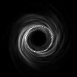
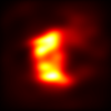
Time-Varying Emission

You can download the sample data from here. This sample data was generated assuming a changing emission image. The video used to generate the results is shown as a log-scale video. We have included data with only thermal error, and data with thermal and atmospheric phase errors. The naming is as follows:

Filename	Property
timevarying_wNoPhaseError	In addition to time-varying changes, only thermal noise is included in visibility measurements
timevarying	In addition to time-varying changes, thermal and phase (atmospheric) errors are included in visibility measurements

Past Challenges

Download the data and see results from the 1st EHT Imaging Challenge HERE
Download the data and see results from the 2nd EHT Imaging Challenge HERE
Download the data and see results from the 3rd EHT Imaging Challenge HERE
Download the data and see results from the 4th EHT Imaging Challenge HERE
Download the data and see results from the 5th EHT Imaging Challenge HERE

Data Formats and Conversion

We have provided data in a number of formats (Text File, UVFITS, OIFITS). You can read more about some of these data formats here. You can convert between formats using the Python EHT Imaging Library.

Download the EHT Imaging Library:

  
 $ git clone https://github.com/achael/eht-imaging.git 
 $ cd eht-imaging

Convert between Data Formats in Python 2.7 using the EHT Imaging Library:

 
import vlbi_imaging_utils as vb
 
# load data from text file and save out as uvfits and oifits 
obs = vb.load_obs_txt('data/challenge_01.txt'); 
obs.save_uvfits('data/challenge_01_out.uvfits');
obs.save_oifits('data/challenge_01_out.oifits');
# save a normalized oifits file with a true total flux of 2.0 Jy 
obs.save_oifits('data/challenge_01_out_normalized.oifits', flux=2.0);

# load data from uvfits file and save out as text file 
obs = vb.load_obs_uvfits('data/challenge_01.uvfits'); 
obs.save_txt('data/challenge_01_out.txt');

# load data from oifits file - oifits does not save polametric quantities 
obs = vb.load_obs_oifits('data/challenge_01.oifits'); 
# load a normalized oifits file with a true total flux of 2.0 Jy 
obs = vb.load_obs_oifits('data/challenge_01_out_normalized.oifits', flux=2.0);

Sample Imaging Script

To help you get started, we provide a script that shows you how you can image the sample data provided above using the Python EHT Imaging Library.

Download the EHT Imaging Library:

  
 $ git clone https://github.com/achael/eht-imaging.git 
 $ cd eht-imaging

Image using Bispectrum Maximum Entropy methods in Python 2.7 using the EHT Imaging Library:

Script that images using Bispectrum Maximum Entropy Methods Ground Truth Image Blurred With Fitted Beam Maximum Entropy Reconstruction

 
import vlbi_imaging_utils as vb
import maxen as mx
import numpy as np
 
# load data from text file 
obs = vb.load_obs_txt('data/challenge_01.txt'); 
 
# specify imaging parameters 
flux = 2.0 # total flux of the source 
fov = 0.00016 # field of view in arcseconds 
npix = 100 # number of pixels 
 
# create the prior used for maximum entropy imaging 
fovrad = fov / 206265.0 # field of view in radians 
emptyprior = vb.make_square(obs, npix, fovrad) 
prior_fwhm = 100*vb.RADPERUAS # Gaussian size in microarcssec
gaussprior = vb.add_gauss(emptyprior, flux, (prior_fwhm, prior_fwhm, 0, 0, 0))
 
# find a best fit image using the maximum entropy method and save out the data 
out = mx.maxen_bs(obs, gaussprior, gaussprior, flux, maxit=50, alpha=100, entropy="gs")

# blur with 1/2 telescope beam 
beamparams=obs.fit_beam() 
outblur = vb.blur_gauss(out, beamparams, 0.5) 

out.save_fits('challenge_01_mxen.fits')
outblur.save_fits('challenge_01_blur.fits')

Questions and Feedback

We are happy to help out with any questions you may have. Please email vlbiimaging@gmail.com with your questions and feedback.